

In Differential calculusDifferential calculus equation there were only differential equations in one dimension to be solved. But there are various occasions were a differential equation of more than just one dimension must be solved.
The equation
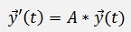
where y and its differentiation appears in form of a vector and A is a matrix, is called a first order homogeneous differential equation system.
To solve this equation let
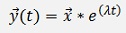
With x as a vector of fixed values and λ a parameter.
Then
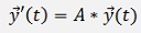
And with the formulation from above:
And y’ replaced
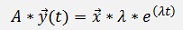
The vector of y on the left side can be replaced as well:

and with some brackets:
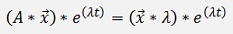

And this is the basic equation for one Eigenvalue and Eigenvector of the matrix A (see Eigenvalues)
That means the equation
Has one solution for the Eigenvalue λ and its Eigenvector x of the matrix A. And if the matrix A has more than one Eigenvalue, the differential equation system has more than one solution to. That means to solve this equation the Eigenvalues and their Eigenvectors of the matrix A must be found.
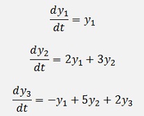
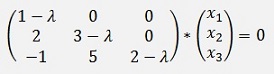
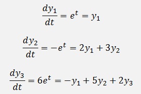
For a sample equation system like:
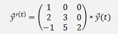
The matrix form is
And for the Eigenvalues the following Determinant shall be 0
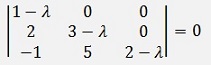
(See Eigenvalue calculation by the roots of the characteristic polynomial)
(o.k. that’s a very simple sample
 )
)
This Determinant is
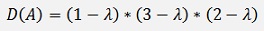
And it becomes 0 if λ = 1 or λ = 2 or λ = 3
To get the Eigenvectors these solutions must be inserted in the equation
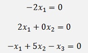
For λ = 1 that is
These equations are under determined and so x1 = 1 can be set arbitrary.
And with this

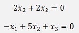
For λ = 2 that is
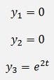
These equations are under determined to. But x1 = 0 and x2 = 0. Only x3 can be set arbitrary. So we can set and

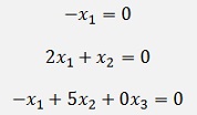
For λ = 3 that is
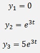
These equations are under determined again and so x2 = 1 can be set and

So we have 3 solutions:
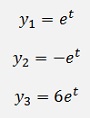
Whit λ = 1:
Whit λ = 2:
Whit λ = 3:
To evaluate this result:
For λ = 1:
o.k.
Such a simple equation can be solved manually. That’s nice to show. But for more complex equations a computer supported approach is required and therefore see Eigenvalue calculation by the roots of the characteristic polynomial)