To compute the Eigenvalues and Eigenvectors of a quadratic matrix the QR decomposition to compute real and complex Eigenvalues is for sure the strongest algorithm. But if there is no need for Eigenvectors, the use of the characteristic polynomial and its roots is an elegant approach to and it is a bit less complex. And if there is still some desire to compute the Eigenvectors, they can still be computed. But this further down

To compute the characteristic polynomial of a n*n matrix
The basic formulation for one Eigenvalue of a matrix A and its Eigenvector is

This can be written as

and as

With λ multiplied by the identity matrix In:

The vector x can be separated

And here the expression in the brackets is a matrix and the entire expression becomes 0 if the Determinant of (A - λ * In) is 0

For a 3*3 matrix this would look like:

Written in an polynomial that’s

(See Matrix determinant and Cramers method for the calculation of a determinant) With the brackets removed this would be the characteristical polynomial.
Of this polynomial the roots are the Eigenvalues. To find these roots by hand might be bearable for a 3*3 matrix. But for higher order matrixes that becomes crazy.
Therefore a recursive implementation of the followning C# function can be used.
double[] CalcDet(TPolynom[,] m, int order)
{
int i, j, k;
double sign = 1.0;
double[] tempPoly = new double[2];
TPolynom dm = new TPolynom(1);
TPolynom tempDet = new TPolynom(2);
if (order <= 2)
{
tempDet.a = m[0, 0].Mult(m[1, 1].a);
tempPoly = tempDet.Sup(m[1, 0].Mult(m[0, 1].a));
return tempPoly;
}
TPolynom[,] mm = new TPolynom[order - 1, order - 1]; // temporary matrix
for (i = 0; i < order - 1; i++) // index for the element of the top row
{
for (j = 0; j < order - 1; j++)
mm[i, j] = new TPolynom(1);
}
for (i = 0; i < order; i++) // index for the element of the first row
{
for (j = 0; j < order - 1; j++) // index that runs down from second row to n
{
for (k = 0; k < order - 1; k++) // index to copy the elements into a sub matrix
{
if (j < i)
{
mm[j, k].Copy(m[k + 1, j].a);
}
else
{
mm[j, k].Copy(m[k + 1, j + 1].a);
}
}
}
tempDet.a = CalcDet(mm, order - 1);
tempPoly = tempDet.Mult(m[0, i].a);
if (sign > 0)
dm.a = dm.Add(tempPoly);
else
dm.a = dm.Sup(tempPoly);
sign = -sign;
}
return dm.a;
}
This function is derived from the same function in mosismath/determinant. It is extended by the functions in the class
public class TPolynom
Whit the functions
public double[] Mult(double[] p2)
public double[] Mult(double p2)
public double[] Divide(double[] b, int order)
public double[] Add(double[] p2)
public double[] Sup(double[] p2)
public void Copy(double[] source)
for the basic math functions with polynomials With the 2 dimensional array p the function CalcDet returns the determinant in a polynomial like:
double[] det = CalcDet(p, ORDER);
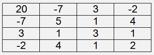
The matrix

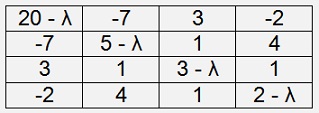
Where p is the matrix A with the diagonal elements subtracted by λ

would have the characteristic polynomial

With the highest power in the first element, the second highest in the second and so on. That’s the first step. The second step is to compute the roots of this polynomial and that’s done by the Bairstow algorithm (see Complex roots of a polynomials )
To compute the complex and real roots of a polynomial
The 4*4 matrix above is symmetrical. That means it only has real Eigenvalues. But not every matrix is symmetrical and a non-symmetrical matrix usually has complex Eigenvalues as well and therefore the characteristical polynomial can have complex roots.
To find complex roots of a polynomial the mosismath/Bairstow algorithm can be used. It finds pairs of complex roots and pairs of real roots like λ2 +(a+b)λ + ab what would be (λ + a)*( λ + b). These pairs of roots must be separated afterwards.
In case the polynomial contains an odd number of real roots, there will be a remaining polynomial at the end what would be the last real root.
The function Findroot(double[] a, int order) from mosismath/Baistow finds all pairs of roots of the polynomial a and places them into the list “root”.
private int FindRoot(double[] a, int order)
{
double bn, bn1, bn2;
double cn, cn1, cn2;
double dxp, xp_old, dxq, xq_old;
r = new SRoot();
int i;
int result = 1;
r.p = -2.0; // Starting point
r.q = -5.0;
dxp = r.p;
dxq = r.q;
while ((Math.Abs(dxp) > 1E-10) && (Math.Abs(dxq) > 1E-10)) // check if we are close enough
{
xp_old = r.p;
xq_old = r.q;
bn2 = a[0];
cn2 = bn2;
bn1 = a[1] + r.p * bn2;
cn1 = bn1 + r.p * cn2;
cn = 0;
bn = 0;
for (i = 2; i < order; i++)
{
bn = r.p * bn1 + r.q * bn2 + a[i];
if (i < order - 1)
{
cn = r.p * cn1 + r.q * cn2 + bn;
if (i < order - 2)
{
cn2 = cn1;
cn1 = cn;
}
bn2 = bn1;
bn1 = bn;
}
}
if (Math.Abs(cn1 * cn1 - cn * cn2) > 1E-30) // nex p and q
{
r.p = r.p + (bn * cn2 - bn1 * cn1) / (cn1 * cn1 - cn * cn2);
r.q = r.q + (bn1 * cn - bn * cn1) / (cn1 * cn1 - cn * cn2);
dxp = r.p - xp_old;
dxq = r.q - xq_old;
}
else
result = -1;
}
if (result > 0)
root.Add(r);
return result;
}
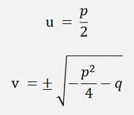
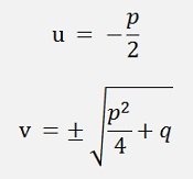
The roots in the list root have the form λ2 – p λ – q = 0 (remark the minus signs). They can be resolved by the mosismath/QuadExt solution.
In case of complex roots the solution is

and the roots are u + jv and u – jv
In case of real roots the solution is

and the roots are u + v and u - v.
In case there is one last real root remaining, a polynomial in the form λ + x will remain in the input polynomial a after calling the Findroot(double[] a, int order). Then the last real root is –x

So. Finally the above 4*4 matrix has the Eigenvalues:
-1.160949791926147
1.173048870316898
6.460514719957084
23.527386201652163
To compute the Eigenvectors to Eigenvalues
If there is a need for the Eigenvectors, they can still be computed by using the complex form of the elimination algorithm by Gauss applied to the formulation

For each Eigenvalue the Eigenvector can be computed with this equation. The only little point to remark is the detail, that the Gaussian elimination algorithm does not like the 0’s on the right side of these equations. But that can easily be avoided by adding 1 on both sides of all equations. In the matrix that would mean to add 1 to all elements in the last column. With λ that would look like:

With this the EigenvectorsEigenvectors to the Eigenvalues become:


